How do you write Integrals(∫,∮) in LaTeX?

The command for displaying an integral sign is \int and the general syntax for typesetting integrals with limits in LaTeX is

\int_{min}^{max}

which types an integral with a lower limit min and upper limit max.

\documentclass{article}
\begin{document}
   The integral of a real-valued function $ f(x) $ with respect to  $ x $ on the closed interval, $ [a, b] $ is denoted as
   \[
   \int_{a}^{b}f(x)\,\mathrm{d}x.
   \]
\end{document}

Output :

The integral sign together with the limits appears differently in the inline mode and the display mode. In the inline mode, the limits appear next to the symbol and in the display mode, the limit appears below and above the summation sign.

There are two commands that are capable of controlling how these limits appear.

First is the \limits command which forcefully pushes the limits below and above the integral sign in all the math modes and the second is the \nolimits command which reverse the effect(forces the limits to stay next to the integral symbol in all math modes).

\documentclass{article}
\begin{document}
  \begin{tabular}{|@{\quad}c@{\quad}|@{\quad}c|}
   \hline 
   \multicolumn{2}{|c|}{\textbf{Integral in math mode}}\\ 
   \hline 
   inline math mode & display math mode\\ 
   \hline 
   $ \int_{k=1}^n $ & $ {\displaystyle \int_{k=1}^n} $\\  
   \hline 
   \multicolumn{2}{|c|}{\textbf{Integral in math mode with} \color{blue}{\textbackslash{}limits}}\\ 
   \hline 
   $ \int\limits_{k=1}^n $ & $ {\displaystyle \int\limits_{k=1}^{n}} $\\  
   \hline 
   \multicolumn{2}{|c|}{\textbf{Integral in math mode with} \color{blue}{\textbackslash{}nolimits} }\\ 
   \hline 
   $ \int\nolimits_{k=1}^n $ & $ {\displaystyle \int\nolimits_{k=1}^{n} }$\\ 
   \hline 
  \end{tabular}
\end{document}

Types of integrals

There are many different types of integrals and the LaTeX amsmath package provides us with the various commands to typeset them as shown in the table below :

At the same time, LaTeX provides us with the esint package which contains even more different types of integrals as we shall be seeing below.

Package can be complemented by two important optional arguments when loading it at the level of the preamble.

The first is nointlimits which causes the limits to be placed in front of the integral sign and the intlimits which places the limits under and above the integral sign. The two optional arguments are loaded in the preamble as follows

\usepackage[nointlimits]{esint} or \usepackage[intlimits]{esint}

Which will produce for example or respectively in your document. Below we have the various commands provided to us by the esint package.

LaTeX command	Name and Output
\int	Single integral → ∫
\iint	Double integral → ∬
\iiint	Triple integral → ∭
\iiiint	Quadruple integral → ⨌
\idotsint	∫…∫
\oint	Contour integral → ∮
\varointclockwise	Clockwise contour integral → ∲
\ointctrclockwise	Counterclockwise contour integral → ∳
\varointctrclockwise	Counterclockwise contour integral →
\ointclockwise	Clockwise contour integral →
\oiint	Closed surface integral →
\varoiint	Closed surface integral →
\sqint	Integral with square path →

Also, we can achieve the volume integral by loading mathdesign together with the charter optional argument.

Below is what you need to add in the preamble (Note that this package conflicts with a few other packages and so should be used with the integral commands that it provides)

\usepackage[charter]{mathdesign}

LaTeX command	Name and Output
\oiiint	Closed volume integral →

Examples

Example 1.

\documentclass{article}
\usepackage{amssymb,esint}
\begin{document}
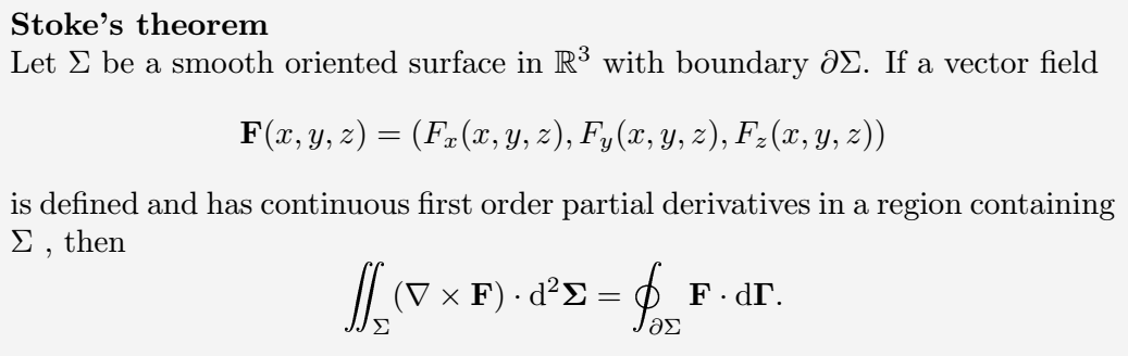
   \textbf{Divergence theorem}\\
   Suppose $ V $ is a subset of $ \mathbb{R}^{n} $ (in the case of $ n = 3 $, $ V $ represents a volume in three-dimensional space) which is compact and has a piecewise smooth boundary $ S $(also indicated with  $ \partial V=S $). If $ F $ is a continuously differentiable vector field defined on a neighborhood of $ V $, then:
   \[
   \iiint_{V} ( \mathbf{\nabla} \cdot \mathbf{F})\,\mathrm{d}V=\oiint_S \mathbf{F} \cdot \mathbf{\hat{n}} \mathrm{d}S
   \]
   The left side is a volume integral over the volume $ V $, the right side is the surface integral over the boundary of the volume $ V $.
\end{document}

Output :

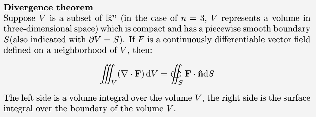
Example 2.

\documentclass{article}
\usepackage{amssymb,esint}
\begin{document}
   \textbf{Stoke's theorem}\\
   Let $ \Sigma $  be a smooth oriented surface in $ \mathbb{R}^3 $ with boundary $ \partial \Sigma  $. If a vector field 
   \[ \mathbf {F} (x,y,z)=(F_{x}(x,y,z),F_{y}(x,y,z),F_{z}(x,y,z)) \]
   is defined and has continuous first order partial derivatives in a region containing $ \Sigma $ , then
   \[
   \iint _{\Sigma }(\nabla \times \mathbf{F})\cdot \mathrm{d}^{2}\mathbf{\Sigma} =\oint_{\partial \Sigma}\mathbf{F} \cdot \mathrm{d}\mathbf{\Gamma}.
   \]
\end{document}

Output :

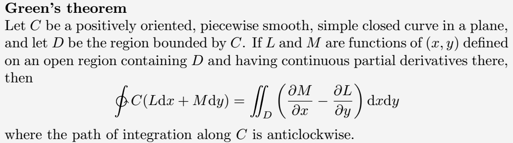
Example 3.

\documentclass{article}
\usepackage{esint}
\begin{document}
   \textbf{Green's theorem}\\
   Let $ C $ be a positively oriented, piecewise smooth, simple closed curve in a plane, and let $ D $ be the region bounded by $ C $. If $ L $ and $ M $ are functions of $ (x, y) $ defined on an open region containing $ D $ and having continuous partial derivatives there, then
   \[
   \ointctrclockwise C(L\mathrm{d}x+M\mathrm{d}y)=\iint _{D}\left(\frac{\partial M}{\partial x}-\frac{\partial L}{\partial y}\right)\mathrm{d}x\mathrm{d}y \] 
   where the path of integration along $ C $ is anticlockwise.
\end{document}

Output :